Spreadsheet Modeling And Decision Analysis 6th Edition Pdf Download UPDATED

Spreadsheet Modeling And Decision Analysis 6th Edition Pdf Download

Basics of Queueing Theory

Many (not all) simulation models are of queueing systems representing a wide variety of real operations. For instance, patients arrive to an urgent-intendance clinic (i.e., they just show up randomly without appointments), and they all must offset sign in, possibly after waiting in a line (or a queue) for a bit; see Figure ii.1.

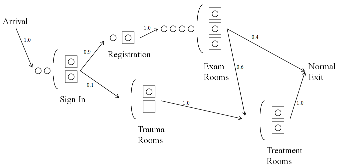
Figure 2.1: A queueing organisation representing and urgent-care clinic

Afterward signing in, patients become either to registration or, if they're seriously ill, go to a trauma room, and could have to wait in queue at either of those places too before being seen. Patients going to the Test room and so either exit the organization, or go to a treatment room (maybe queueing at that place first) and and so go out. The seriously ill patients that went to a trauma room then all go to a treatment room (perhaps later queueing at that place too), and then they leave. Questions for designing and operating such a facility might include how many staff of which type to have on duty during which time periods, how large the waiting room should exist, how patient waiting-room stays would be affected if the doctors and nurses decreased or increased the fourth dimension they tend to spend with patients, what would happen if 10% more patients arrived, and what might exist the touch on of serving patients in an order co-ordinate to some mensurate of acuity of their presented condition instead of beginning-come up, showtime served.

This brusk chapter will cover just the basics of queueing theory (not queueing simulation), since familiarity with this material and the terminology is of import for developing many simulation models. The relatively elementary mathematical formulas from elementary queueing theory can also bear witness valuable for verification of simulation models of queueing systems (helping to determine that the simulations are correct). Queueing-theory models tin can do that past providing a benchmark against which simulation results can exist compared, if the simulation model is simplified (probably unrealistically) to lucifer the more stringent assumptions of queueing theory (east.g., assuming exponential probability distributions even though such is not true for the real organisation we're simulating). If the (simplified) simulation model approximately agrees with the queueing-theoretic results, so we take better conviction that the simulation model's logic, at least, is right. Equally we develop our Simio simulation models in later chapters, we'll do this repeatedly, which is helpful since simulation "code" can exist quite circuitous and thus quite difficult to verify.

Queueing theory is an enormous subject, and has been studied mathematically since at to the lowest degree 1909, at first by A.K. Erlang in connection with how the recently-invented "phone" systems in Copenhagen, Denmark might be designed and perform ((Erlang 1909), (Erlang 1917)). There are many entire books written on information technology (e.m., (Gross et al. 2008), (Kleinrock 1975)), besides every bit extensive chapters in more general books on probability and stochastic processes (east.grand. (Ross 2010)) or on other application-oriented topics similar manufacturing (e.g. (Askin and Standridge 1993)); a web search on "queueing theory" returned more than than 1.four 1000000 results. Thus, nosotros make no attempt hither to requite whatsoever sort of complete treatment of the subject field; rather, nosotros're just trying to introduce some terminology, give some basic results, contrast queueing theory with simulation via their relative strengths and weaknesses, and provide some specific formulas that we'll use in later capacity to aid verify our Simio simulation models.

In this affiliate (and really, in the whole book), we assume that you're already familiar with bones probability, including:

• The foundational ideas of a probabilistic experiment, the sample space for the experiment, and events.

• Random variables (RVs), both the detached and continuous flavors.

• Distributions of RVs — probability mass functions (PMFs) for discrete, probability density functions (PDFs) for continuous, and cumulative distribution functions (CDFs) for both flavors.

• Expected values of RVs and their distributions (a.k.a. expectations or just ways), variances, and how to use PMFs, PDFs, and CDFs to compute probabilities that RVs will land in intervals or sets.

• Independence (or lack thereof) between RVs.

If not, so you lot should first go back and review those topics before reading on.

In this chapter, and elsewhere in the book, we'll ofttimes refer to specific probability distributions, like the exponential, uniform, triangular, etc. In days gone past books using probability notions independent lots of pages of distribution facts similar definitions of PMFs, PDFs, and giving CDFs, expected values, variances, then on, for many distributions. But this volume does not have such a compendium since that material is readily bachelor elsewhere, including the Simio documentation itself (described in Section six.ane.iii), and on-line, such as https://en.wikipedia.org/wiki/List_of_probability_distributions, which in turn has links to web pages on well over 100 specific univariate distributions. Encyclopedic books, such as (Johnson, Kotz, and Balakrishnan 1994), (Johnson, Kotz, and Balakrishnan 1995), (Johnson, Kemp, and Kotz 2005), and (Evans, Hastings, and Peacock 2000), have been compiled. References to further material on distributions are in Section half-dozen.1.3, forth with some discussion of their backdrop, such equally ranges.

In Section ii.1 we'll describe the general structure, terminology, and notation for queueing systems. Section 2.2 states some important relationships amongst unlike output functioning metrics of many queueing systems. We'll quote a few specific queueing-arrangement output results in Section two.three, and briefly draw how to deal with networks of queues in Section 2.4. Finally, in Department 2.5 we'll compare and contrast queueing theory vs. simulation as analysis tools, and show that each has pros and cons that dovetail nicely with each other (though on balance, we still like simulation better well-nigh of the time).

Queueing-System Structure and Terminology

A queueing organization is ane in which entities (like customers, patients, jobs, or messages) go far, get served either at a unmarried station or at several stations in plow, might have to wait in one or more queues for service, and and so may leave (if they do leave the system is chosen open, but if they never leave and merely keep circulating around inside the system it's called closed).

The urgent-care clinic described earlier, and in Figure 2.i, is modeled every bit an open queueing system. There are 5 split up service stations (Sign In, Registration, Trauma Rooms, Exam Rooms, and Handling Rooms), each of which could be called a node in a network of multiserver queueing nodes (Registration has merely a single server, but that'due south a special case of multiserver). If there are multiple individual parallel servers at a queueing node (due east.thousand., three for Exam Rooms), a single queue "feeds" them all, rather than having a separate queue for each unmarried server, and we ordinarily assume that the private servers are identical in terms of their capabilities and service rates. The numbers by the arcs in Figure ii.i give the probabilities that patients volition follow those arcs. When coming out of a station where at that place's a pick about where to go next (out of Sign In and Exam Rooms) nosotros need to know these probabilities; when coming out of a station where all patients go to the aforementioned next station (out of Arrival, Registration, Trauma Rooms, Handling Rooms) the i.0 probabilities noted in the arcs are obvious, but we show them anyway for abyss. Though terminology varies, nosotros'll say that an entity is in queue if it'south waiting in the line merely not in service, so right now at the Exam Rooms in Figure ii.1 there are four patients in queue and 7 patients in the Examination-Room organization; there are three patients in service at the Exam Rooms.

When a server finishes service on an entity and there are other entities in queue for that queueing node, we demand to determine which specific entity in queue volition be chosen to move into service next — this is called the queue bailiwick. Yous're no doubt familiar with first-come, first-served (better known in queueing as first-in, first-out, or FIFO), which is mutual and might seem the "fairest." Other queue disciplines are possible, though, like last-in, kickoff-out (LIFO), which might correspond the experience of chilled plates in a stack waiting to be used at a salad bar; clean plates are loaded onto the summit, and taken from the meridian as well past customers. Some queue disciplines use priorities to pay attending to differences among entities in the queue, like shortest-job-start (SJF), too called shortest processing time (SPT). With an SJF queue subject, the side by side entity chosen from the queue is i whose processing time will be lowest amongst all those and then in queue (you lot'd have to know the processing times beforehand and assign them to individual entities), in an attempt to serve quickly those jobs needing merely a little service, rather than making them wait backside jobs requiring long service, thereby hopefully improving (reducing) the average time in queue across all entities. Compassion the poor big job, though, as information technology could be stuck most the dorsum of the queue for a very long time, so whether SJF is "better" than FIFO might depend on whether you care more about average time in arrangement or maximum (worst) time in system. A kind of opposite of SJF would exist to take values assigned to each entity (maybe profit upon exiting service) and you'd similar to choose the next task from the queue as the one with the highest value (time is money, you know). In a wellness-care system similar that in Effigy ii.1, patients might be initially triaged into several vigil levels, and the next patient taken from a queue would one in the well-nigh serious vigil-level queue that's non-empty; within each vigil-level queue a tie-breaking rule, such as FIFO, would be needed to select amid patients at the same acuity level.

Several performance measures (or output metrics) of queueing systems are often of interest:

• The fourth dimension in queue is, equally you'd guess, the fourth dimension that an entity spends waiting in line (excluding service time). In a queueing network like Figure 2.1, we could speak of the time in queue at each station separately, or added up for each patient over all the private times in queue from inflow to the system on the upper left, to go out on the far right.

• The time in organization is the time in queue plus the time in service. Again, in a network, nosotros could refer to time in system at each station separately, or overall from arrival to get out.

• The number in queue (or queue length) is the number of entities in queue (over again, non counting any entities who might be in service), either at each station separately or overall in the whole system. Correct now in Figure ii.one at that place are two patients in queue at Sign In, one at Registration, four at Exam Rooms, and none at both Trauma Rooms and Treatment Rooms; there are seven patients in queue in the whole organization.

• The number in arrangement is the number of entities in queue plus in service, either at each station separately or overall in the whole arrangement. Right at present in Figure 2.1 there are four patients in organization at Sign In, two at Registration, 7 at Exam Rooms, one at Trauma Rooms, and two at Treatment Rooms; there are 16 patients in the whole arrangement.

• The utilization of a server (or group of parallel identical servers) is the time-boilerplate number of individual servers in the group who are busy, divided by the total number of servers in the grouping. For case, at Test Rooms there are three servers, and if we let \(B_E(t)\) be the number of the individual exam rooms that are busy (occupied) at any fourth dimension \(t\), then the utilization is \[\begin{equation} \frac{\int_0^h B_E(t) dt} {3h}, \tag{2.1} \finish{equation}\] where \(h\) is the length (or horizon) of fourth dimension for which nosotros observe the arrangement in performance.

With only very few exceptions, the results available from queueing theory are for steady-state (or long-run, or infinite-horizon) conditions, as time (real or imitation) goes to infinity, and frequently just for steady-state averages (or ways). Hither'south mutual (though non universal) annotation for such metrics, which we'll use:

• \(W_q=\) the steady-state boilerplate time in queue (excluding service times) of entities (at each station separately in a network, or overall across the whole network).

• \(W=\) the steady-state average fourth dimension in organisation (including service times) of entities (again, at each station separately or overall).

• \(L_q=\) the steady-state average number of entities in queue (at each station separately or overall). Note that this is a time average, non the usual boilerplate of a discrete list of numbers, and so might require a scrap more caption. Allow \(L_q(t)\) exist the number of entities in queue at fourth dimension instant \(t\), so \(L_q(t) \in \{0, one, 2, \ldots\}\) for all values of continuous time \(t\). Imagine a plot of \(L_q(t)\) vs.\(t\), which would be a piecewise-abiding bend at levels 0, ane, two, … , with jumps up and down at those time instants when entities enter and go out the queue(south). Over a finite fourth dimension horizon \([0, h]\), the fourth dimension-average number of entities in queue(south) (or the time-average queue length if we're talking about but a single queue) will be \(\overline{L_q}(h) = \int_0^h L_q(t) dt/h\), which is a weighted boilerplate of the levels 0, 1, ii, … of \(L_q(t)\), with the weights beingness the proportion of fourth dimension that \(L_q(t)\) spends at each level. Then \(L_q = \lim_{h \rightarrow \infty} \overline{L_q}(h)\).

• \(L=\) the steady-state average number of entities in system (at each station separately or overall). Every bit with \(L_q\), this is a fourth dimension average, and is indeed divers similarly to \(L_q\), with \(L(t)\) defined every bit the number of entities in the system (in queue plus in service) at fourth dimension \(t\), and and so dropping the subscript \(q\) throughout the discussion.

• \(\rho=\) the steady-state utilization of a server or grouping of parallel identical servers, typically for each station separately, as defined in equation (2.1) in a higher place for the Exam-Rooms case, but after letting \(h \rightarrow \infty\).

Much of queueing theory over the decades has been devoted to finding the values of these v steady-land average metrics, and is certainly far beyond our scope here. We will mention, though, that due to its very special property (the memoryless property), the exponential distribution is disquisitional in many derivations and proofs. For instance, in the simplest queueing models, interarrival times (times between the arrivals of two successive entities to the organization) are often causeless to have an exponential distribution, every bit are individual service times. In more advanced models, those distributions tin be generalized to variations of the exponential (like Erlang, an RV that is the sum of independent and identically distributed (IID) exponential RVs), or even to general distributions; with each step in the generalization, though, the results become more complex both to derive and to apply.

Finally, there'south a standard notation to describe multiserver queueing stations, sometimes called Kendall's annotation, which is meaty and convenient, and which nosotros'll utilise: \[A/B/c/k.\] An indication of the inflow process or interarrival-time distribution is given by \(A\). The service-time RVs are described by \(B\). The number of parallel identical servers is \(c\) (so \(c=3\) for the Test Rooms in Figure ii.1, and \(c=1\) for Registration). The capacity (i.e., upper limit) on the system (including in queue plus in service) is denoted by \(k\); if in that location's no capacity limit (i.due east., \(g = \infty\)), then the \(/\infty\) is normally omitted from the end of the notation. Kendall's notation is sometimes expanded to signal the nature of the population of the input entities (the calling population), and the queue discipline, merely nosotros won't need whatever of that. Some item choices for \(A\) and \(B\) are of note. Ever, \(M\) (for Markovian, or perhaps memoryless) means an exponential distribution for either the interarrival times or the service times. Thus the \(M/M/1\) queue has exponential interarrival times, exponential service times (causeless independent of the interarrival times), and simply a single server; \(M/M/3\) would draw the Exam Rooms component in Figure 2.i if we knew that the interarrival times to it (coming out of Registration) and the Test-Room service times were exponential. For an Erlang RV equanimous of the sum of \(chiliad\) IID exponential RVs, \(E_m\) is mutual notation, so an \(Thousand/E_3/2/ten\) system would have exponential interarrival times, iii-Erlang service times, two parallel identical servers, and a limit of ten entities in the arrangement at whatever i time (so a maximum of eight in the queue). The notation \(Yard\) is commonly used for \(A\) or \(B\) when nosotros want to allow a general interarrival-time or service-time distribution, respectively.

Picayune's Law and Other Relations

There are several important relationships amidst the steady-land average metrics \(W_q\), \(W\), \(L_q\), and \(L\), defined in Section two.1, which brand computing (or estimating) the rest of them fairly simple if you know (or tin can guess) any 1 of them. In this section we're thinking primarily of just a unmarried multiserver queueing station (like just the Exam Rooms in Effigy 2.1 in isolation). Further note nosotros'll need is \(\lambda\) = the inflow rate (which is the reciprocal of the expected value of the interarrival-time distribution), and \(\mu\) = the service rate of an individual server, non a group of multiple parallel identical servers (so \(\mu = 1/Eastward(S)\), where \(S\) is an RV representing an entity's service fourth dimension in an individual server).

The most important of these relationships is Little's police force, the first version of which was derived in (Little 1961), but information technology'southward been generalized repeatedly, e.g. (Stidham 1974); recently it historic its 50th anniversary ((Fiddling 2011)). Stated simply, Trivial's police is just \[L=\lambda W\] with our note from in a higher place. In our awarding nosotros'll consider this just for a single multiserver queueing station, only be aware that it does apply more generally. The remarkable matter almost Little's law is that it relates a time average (\(50\) on the left-hand side) to an entity-based observational average (\(Due west\) on the right-manus side).

More than physically intuitive than Piffling's law is the relationship \[W = W_q + E(Due south),\] where we presume that we know at to the lowest degree the expected value \(Due east(South)\) of the service-time distribution, if non the whole distribution. This simply says that your expected time in system is your expected fourth dimension in queue plus your expected service time. This relationship, together with \(L=\lambda West\) and \(L_q=\lambda W_q\), allows yous to get whatsoever of \(W_q\), \(W\), \(L_q\), and \(L\) if you lot know just one of them. For instance, if you know (or can estimate) \(W_q\), then only substituting yields \(L = \lambda (W_q + E(S))\); as well, if you know \(L\), then subsequently a little algebra you get \(W_q = L/\lambda - Due east(Due south)\).

Specific Results for Some Multiserver Queueing Stations

In this section nosotros'll just list formulas from the literature for a few multiserver queueing stations, i.e., something like the Exam Rooms in Figure 2.1, rather than an unabridged network of queues overall as shown across that entire effigy. Remember, you tin can use Little's law and other relations from Section 2.2 to go the other typical steady-state boilerplate metrics. Throughout, \(\rho = \lambda/(c \mu)\) is the utilization of the servers equally a group (recall that \(c\) is the number of parallel identical servers at the queueing station); higher values of \(\rho\) generally portend more congestion. For all of these results (and throughout nigh of queueing theory), we demand to assume that \(\rho < ane\) (\(\rho\le 1\) isn't good enough) in order for whatever of these results to exist valid, since they're all for steady state, so we must know that the system will not "explode" over the long run with the number of entities present growing without bound — the servers, as a grouping, demand to exist able to serve entities at least as fast as they're arriving.

In addition to just the four specific models considered here, at that place are certainly other such formulas and results for other queueing systems, bachelor in the vast queueing-theory literature mentioned at the get-go of this chapter. However, they do tend to get quite complicated quite quickly, and in some cases are not really airtight-form formulas, but rather equations involving the metrics you want, which you and then need to "solve" using various numerical methods and approximations (as is actually the case with our fourth instance below).

M/M/1

Perhaps the simplest of all queueing systems, we have exponential interarrival times, exponential service times, and just a unmarried server.

The steady-state average number in system is \(L = \rho/(1-\rho)\). Remember that \(\rho\) is the mean inflow rate \(\lambda\) divided past the hateful service rate \(\mu\) if there'due south only a unmarried server. Certainly, \(50\) can be expressed in dissimilar means, similar \[L = \frac{\lambda}{1/Eastward(S) - \lambda}.\] If we know \(L\), nosotros can so use the relations in Section 2.two to compute the other metrics \(W_q\), \(W\), and \(L_q\).

Yard/M/c

Again, both interarrival times and services times follow exponential distributions, but now we take \(c\) parallel identical servers being fed by a single queue.

Showtime, let \(p(north)\) exist the probability of having \(n\) entities in the system in steady state. The only i of these we really demand is the steady-country probability that the organisation is empty, which turns out to be \[ p(0) = \frac{i} {\frac{(c \rho)^c}{c! (one-\rho)} + \sum_{north=0}^{c-1}\frac{(c \rho)^n}{n!}}, \] a picayune complicated merely is just a formula that can be computed, perhaps even in a spreadsheet, since \(c\) is finite, and ofttimes fairly small. (For any positive integer \(j\), \(j! = j \times (j-1) \times (j-ii) \times \cdots \times ii \times ane\), and is pronounced "\(j\) factorial" — not by shouting "\(j\)." Mostly for convenience, \(0!\) is just defined to be 1.) And so, \[ L_q = \frac{\rho(c \rho)^c p(0)} {c! (1-\rho)^2}, \] from which you could go, for example, \(Fifty = L_q + \lambda/\mu\) along with the other metrics via the relationships in Section ii.2.

Though the formulas above for the \(Yard/G/c\) are all airtight-form (i.e., yous tin can in principle plug numbers into them), they're a little complicated, especially the summation in the denominator in the expression for \(p(0)\) unless \(c\) is very small. So nosotros provide a modest command-line program mmc.exe (meet Appendix Department C.iv.2 for the download URL), to do this for values that yous specify for the arrival rate \(\lambda\), the service rate \(\mu\), and the number of servers \(c\). To invoke mmc.exe y'all need to run the Microsoft Windows Control Prompt window (usually via the Windows Commencement push button, then Programs or All Programs, then in the Accessories folder). It's probably simplest to move the mmc.exe file to the "root" bulldoze (usually C:) on your system, and then in the Command Prompt window, type cd .. repeatedly until the prompt reads simply C:\(\backslash >\). If you then type just mmc at the prompt you lot'll get a response telling yous what the syntax is, as shown at the top of Figure two.two. Then, type mmc followed by the values you desire for \(\lambda\), \(\mu\), and \(c\), separated by whatever number of blank spaces. The plan responds with the steady-state queueing metrics for this system, assuming that the values yous specified result in a stable queue, i.e., values for which \(\rho < 1\). The resulting metrics are all for steady-state, using whatever fourth dimension units you used for your input parameters (of course, \(\lambda\) and \(\mu\) must use the aforementioned time units, merely that time unit could be anything and is not needed by mmc.exe).

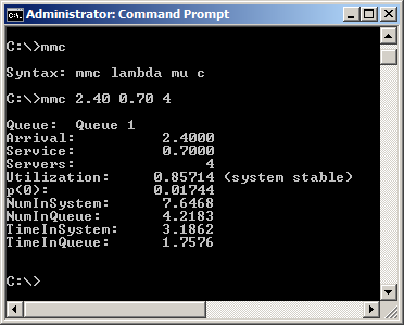
Figure 2.ii: Example of using the mmc.cmd command-line program.

If y'all are a Python user, yous can find a Python mmc module and examples at https://github.com/auie86/mmc. In add-on to solving single-server systems, this module can be used to solve Jackson Network models discussed in Section ii.4.

M/1000/1

This model once once again has exponential interarrival times, simply now the service-time distribution can be annihilation; however, we're back to only a single server. This might be more realistic than the \(Grand/Thousand/i\) since exponential service times, with a mode (most likely value) of zero, are usually far-fetched in reality.

Let \(\sigma\) be the standard difference of the service-time RV \(S\), and so \(\sigma^ii\) is its variance; recall that \(E(South) = ane/\mu\). Then \[ W_q = \frac{\lambda(\sigma^2 + one/\mu^2)}{2(one - \lambda/\mu)}. \] From this (known every bit the Pollaczek-Khinchine formula), yous tin use Little's law and the other relations in Section ii.2 to get boosted output metrics, like \(L\) = the steady-state average number in system.

Note that \(W_q\) here depends on the variance \(\sigma^two\) of the service-time distribution, and non just on its hateful \(1/\mu\); larger \(\sigma^2\) implies larger \(W_q\). Even the occasional extremely long service time tin can necktie upwardly the single server, and thus the system, for a long time, with new entities arriving all the while, thus causing congestion to build up (as measured by \(W_q\) and the other metrics). And the college the variance of the service fourth dimension, the longer the right tail of the service-time distribution, and thus the amend the adventure of encountering some of those extremely long service times.

Thousand/K/1

This last example is a kind of reverse of the preceding one, in that now interarrival times can follow any distribution (of course, they have to be positive to make sense), but service times are exponential. Nosotros only argued that exponential service times are far-fetched, only this supposition, especially its memoryless property, is needed to derive the results below. And, at that place's just a single server. This model is more complex to analyze since, unlike the prior three models, knowing the number of entities present in the system is not enough to predict the futurity probabilistically, because the non-exponential (and thus non-memoryless) interarrival times imply that nosotros too need to know how long it's been since the most recent inflow. Every bit a result, the "formula" isn't really a formula at all, in the sense of being a closed-grade plug-and-chug situation. For more on the derivations, see, for case, (Gross et al. 2008) or (Ross 2010).

Let \(g(t)\) be the density function of the interarrival-time distribution; we'll assume a continuous distribution, which is reasonable, and once more, taking on simply positive values. Recall that \(\mu\) is the service rate (exponential hither), and then the mean service time is \(ane/\mu\). Let \(z\) be a number between 0 and 1 that satisfies the integral equation

\[\begin{equation} z = \int_0^{\infty} e^{-\mu t (one - z)} g(t) dt. \tag{2.2} \end{equation}\]

Then \[ Westward = \frac{1}{\mu (1 - z)}, \] and from that, as usual, we can get the other metrics via the relations in Section 2.2.

And then the question is: What's the value of \(z\) that satisfies equation (two.2)? Unfortunately, (2.2) generally needs to be solved for \(z\) by some sort of numerical method, such every bit Newton-Raphson iterations or another root-finding algorithm. And the task is complicated by the fact that the right-paw side of (two.2) involves an integral, which itself has under it the variable \(z\) we're seeking!

So in general, this is not exactly a "formula" for \(West\), but in some particular cases of the interarrival-time distribution, we might exist able to manage something. For example, if interarrivals have a continuous uniform distribution on \([a,b]\) (with \(0 \le a < b\)), then their PDF is \[ g(t) = \left\{ \begin{assortment}{l 50} i/(b-a) & \quad \mbox{if $a \le t \le b$}\\ 0 & \quad \mbox{otherwise}\\ \end{array} \right.. \] Substituting this into (2.two) results in \[ z = \int_a^b e^{-\mu t (1 - z)} \frac{1}{b-a} dt, \] which, after a little calculus and algebra, turns out to corporeality to \[\begin{equation} z = -\frac{ane}{\mu (b-a)(1-z)}\left[ east^{-\mu(1-z)b} - e^{-\mu(i-z)a}\right], \tag{2.3} \stop{equation}\] and this can exist solved for \(z\) by a numerical method.

Microsoft Excel'due south built-in Goal Seek adequacy, basically a numerical root-finder, might piece of work. In Excel 2007/2010 Goal Seek is on the Data ribbon/tab, under the What-If Analysis button; in other versions of Excel it may be located elsewhere. In the file Uniform_M_1_queue_numerical_solution.xls, which you tin download as specified in Appendix C, we've set this up for this Uniform/\(1000/1\) queue; come across Effigy 2.three.

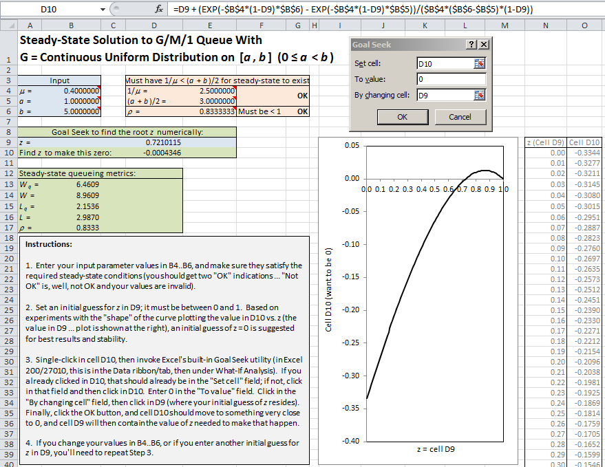
Effigy 2.3: Excel spreadsheet using Goal Seek to solve for stead-state queueing metrics.

The formula in cell D10 (showing at the top of the figure) contains equation (ii.three), except written every bit its left-hand side minus its correct-paw side, and then we use Goal Seek to find the value of \(z\) (in cell D9) that makes this deviation in cell D10 (approximately) 0. You need to supply an initial "guess" at the root-finding value of \(z\) (which must be between 0 and 1) and enter your guess in cell D9; based on experimentation with the shape of the curve in cell D10 as a function of \(z\) in prison cell D9, it appears that initializing with \(z = 0\) in jail cell D9 provides the most robust and stable results. The completed Goal Seek dialog is shown, and the results on the left are afterward information technology has run to completion. After approximating the required solution for \(z\) and confirming that jail cell D10 is (close to) 0, the spreadsheet besides computes the standard steady-state queueing metrics. The text box at the bottom contains more detailed instructions for use of this spreadsheet model.

Queueing Networks

Queueing networks are composed of nodes, each being a multiserver queueing station (like Registration and Treatment Rooms in the urgent-care clinic of Effigy 2.1), and connected past arcs representing possible paths of entity travel from one node to another (or from outside the organization to a node, or from a node to exit the system). Entities can enter from outside the arrangement into any node, though in our clinic they enter merely to the Sign In node. Entities can besides exit the system from whatever node, as they do from the Exam Rooms and Handling Rooms nodes in our clinic. Internally, when an entity leaves a node it can go to any other node, with branching probabilities as in Figure 2.one; from Sign In they go to Registration with probability 0.ix, and to Trauma Rooms with probability 0.1, etc. It's possible that all entities exiting a node go to the same place; such is the case out of the Registration and Trauma Rooms nodes.

We'll presume that all arrival processes from outside are independent of each other with exponential interarrival times (called a Poisson process since the number of entities arriving in a fixed time period follows the discrete Poisson distribution); in our dispensary nosotros accept simply one arrival source from exterior, and all entities from it go to the Sign In node. We'll farther presume that the service times everywhere are exponentially distributed, and independent of each other, and of the input inflow processes. And, we presume that all queue capacities are infinite. Finally, we'll assume that the utilization (a.m.a. traffic intensity) \(\rho\) at each node is strictly less than one, so that the system does not explode anywhere in the long run. With all these assumptions, this is chosen a Jackson network (starting time adult in (Jackson 1957)), and a lot is known nigh it.

In our clinic, looking at but the Sign In node, this is an \(M/M/ii\) with arrival rate that we'll denote \(\lambda_{\textrm{SignIn}}\), which would need to be given (so the interarrival times are IID exponential with mean \(one/\lambda_{\textrm{SignIn}}\)). Remarkably, in stable \(Thou/One thousand/c\) queueing stations, the output is as well a Poisson process with the same rate as the input rate, \(\lambda_{\textrm{SignIn}}\) in this example. In other words, if you stand at the go out from the Sign-In station, you'll see the aforementioned probabilistic behavior that you come across at the entrance to it. Now in this case that output stream is split by an independent toss of a (biased) coin, with each patient's going to Registration with probability 0.ix, and to Trauma Rooms with probability 0.1. And so nosotros have two streams going out, and information technology turns out that each is likewise an contained Poisson process (this is chosen decomposition of a Poisson process), and at rate \(0.9\lambda_{\textrm{SignIn}}\) into Registration and \(0.i\lambda_{\textrm{SignIn}}\) into Trauma Rooms. Thus Registration tin can be analyzed as an \(M/M/ane\) queue with arrival rate \(0.9\lambda_{\textrm{SignIn}}\), and Trauma Rooms can be analyzed equally an \(M/Chiliad/2\) queue with inflow charge per unit \(0.1\lambda_{\textrm{SignIn}}\). Furthermore, all three of the nodes we've discussed and then far (Sign In, Registration, and Trauma Rooms) are probabilistically independent of each other.

Proceeding in this way through the network, we tin analyze all the nodes equally follows:

• Sign In: \(Thou/1000/2\) with inflow rate \(\lambda_{\textrm{SignIn}}\).

• Registration: \(M/M/1\) with inflow rate \(0.nine\lambda_{\textrm{SignIn}}\).

• Trauma Rooms: \(Grand/1000/two\) with arrival rate \(0.1\lambda_{\textrm{SignIn}}\).

• Exam Rooms: \(M/M/3\) with arrival rate \(0.9\lambda_{\textrm{SignIn}}\).

• Handling Rooms: \(Chiliad/One thousand/2\) with arrival rate \[(0.nine)(0.vi)\lambda_{\textrm{SignIn}} + 0.ane\lambda_{\textrm{SignIn}} = 0.64\lambda_{\textrm{SignIn}}.\] The incoming process to Treatment Rooms is called the superposition of two independent Poisson processes, in which case we simply add their rates together to get the effective full incoming rate (and the superposed process is again a Poisson process).

So for each node separately, we could use the formulas for the \(Thousand/M/c\) case (or the command-line program mmc.exe) in Department 2.3 to find the steady-state boilerplate number and times in queue and system at each node separately.

You can do the aforementioned sort of matter to become the utilizations (traffic intensities) at each node separately. Nosotros know from the above list what the incoming charge per unit is to each node, and if we know the service charge per unit of each individual server at each node, we can compute the utilization there. For instance, let \(\mu_{\textrm{Examination}}\) be the service charge per unit at each of the three parallel independent servers at Exam Rooms. Then the "local" traffic intensity at Exam Rooms is \(\rho_{\textrm{Test}} = 0.9\lambda_{\textrm{SignIn}}/(3\mu_{\textrm{Exam}})\). Really, these utilization calculations remain valid for any distribution of interarrival and service-times (not just exponential), in which case the arrival and service rates are defined as simply the reciprocals of the expected value of an interarrival and service-time RV, respectively.

As mentioned higher up, though our urgent-care-clinic example doesn't have it, at that place could be more Poisson input streams from outside the organisation arriving directly into any of the nodes; the overall effective input rate to a node is just the sum of the private input rates coming into it. There could also exist self-loops; for example out of Handling Rooms, it could be that only 80% of patients exit the system, and the other 20% loop directly back to the input for Treatment Rooms (presumably for further treatment); in such a case, it may be necessary to solve a linear equation for, say, \(\lambda_{\textrm{TreatmentRooms}}\). For the assay of this section to remain valid, though, we do need to ensure that the "local" traffic intensity at each of the nodes stays strictly beneath 1. An example of a a generic network with these characteristics is given side by side.

Consider the queueing network shown in Figure 2.four.

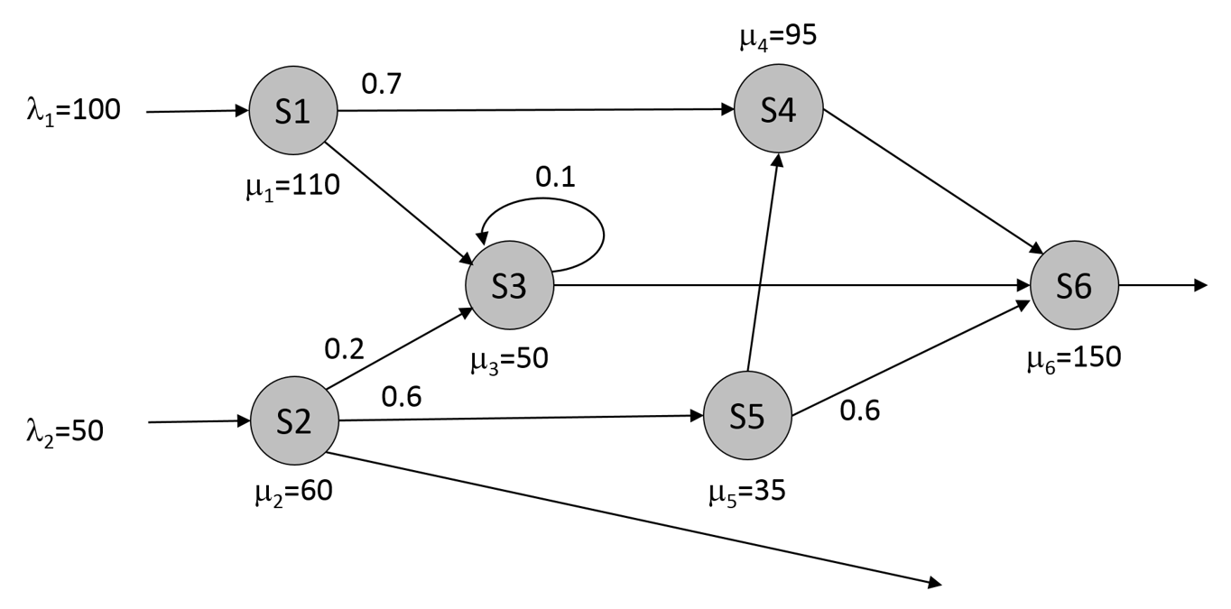
Figure 2.4: Queueing network example. Assume that \(c=ane\) for all stations.

Our interest is in determining the steady-state values for the average number of entities in the system (\(L\)), the average time that an entity spends in the arrangement (\(W\)) and the server traffic intensities (\(\rho_i\)). The outset stride is to make up one's mind the arrival rates for each server. If a server's traffic intensity is strictly less than 1, the departure rate is exactly the arrival rate – we'll assume that this is true for all servers at present and volition verify this as nosotros go. The arrival rates can be computed as: \[\brainstorm{align*} \lambda_1 &= 100 \\ \lambda_2 &= fifty \\ \lambda_3 &= \left(\frac{1}{0.9}\right)(0.3\lambda_1+0.2\lambda_2) \\ \lambda_4 &= 0.7\lambda_1+0.four\lambda_5 \\ \lambda_45 &= 0.6\lambda_2 \\ \lambda_6 &= \lambda_4+0.nine\lambda_3+0.6\lambda_5 \end{align*}\] Given the inflow rates, the service rates shown in Figure 2.four, and the assumption that \(c=1\) for all servers, we can apply the formulae from Department ii.3 to find \(L_i\), \(W_i\), and \(\rho_i\) for each server, \(i\) (encounter Table ii.1).

Table 2.1: Individual station solutions for the network.

	one	2	3	4	5	6
\(\lambda_j\)	100.00	l.00	44.44	82.00	thirty.00	140.00
\(\mu_j\)	110.00	sixty.00	50.00	95.00	35.00	150.00
\(\rho_j\)	0.91	0.83	0.89	0.86	0.86	0.93
\(L_j\)	10.00	5.00	8.00	6.31	6.00	14.00
\(W_j\)	0.ten	0.10	0.18	0.08	0.20	0.ten

Since all of the local traffic intensities are strictly less that ane (the assumption that we made earlier in order to discover the arrival rates), we can discover the overall average number in system, \(L\) and overall average fourth dimension in organization \(Due west\) for the network as:

\[\begin{align*} L &= \sum_{j=1}^vi L_i \\ W &= \frac{L}{\lambda_1 + \lambda_2} \finish{align*}\]

As we volition meet later on in the book, this blazon of assay tin exist very useful for model verification even if the standard queueing assumptions aren't met for a given system that we wish to simulate.

Queueing Theory vs. Simulation

The nice affair well-nigh queueing-theoretic results is that they're exact, i.due east., not subject field to statistical variation (though in some cases where numerical analysis might be involved to observe the solution, as in Department two.three.4 for the \(G/M/ane\) queue, at that place could be roundoff error). As you'll soon see, simulation results are not verbal, and do have statistical uncertainty associated with them, which we do demand to admit, mensurate, and address properly.

But queueing theory has other shortcomings of its own, mostly centered around the assumptions we need to make in order to derive formulas such every bit those in Section 2.iii. In many real-world situations those assumptions will probable be simply wrong, and it'southward hard to say what touch on that might have on definiteness of the results, and thus model validity. Bold exponential service times seems particularly unrealistic in most situations, since the mode of the exponential distribution is aught — when y'all go to, say, drome security, exercise you recollect that it's virtually probable that your service time will be very close to zero, as opposed to having a well-nigh likely value of some number that's strictly greater than zero? And every bit we mentioned, such results are near always but for steady-country operation metrics, so don't tell you much if you're interested in short-term (or finite-horizon or transient) performance. And, queueing-theoretic results are not universally available for all interarrival-time and service-time distributions (call up the mathematical convenience of the memoryless exponential distribution), though approximation methods can exist quite authentic.

Simulation, on the other hand, tin nigh easily deal with short-term (or finite-horizon) fourth dimension frames. In fact, steady-state is harder for simulation since we have to run for very long times, and also worry virtually biasing effects of initial conditions that are uncharacteristic of steady country. And when simulating, we can use whatever interarrival- and service-time distributions seem appropriate to fit the real arrangement we're studying (meet Sections 6.1 and half-dozen.2), and in item we have no need to presume that annihilation has an exponential distribution unless information technology happens to appear that way from the real-world data. Thus, we experience that simulation models stand a amend risk of being more than realistic, and thus more than valid, models of reality, non to mention that their structure can go far beyond standard queueing models into corking levels of complexity that render completely hopeless whatever kind of exact mathematical analysis. The only existent downside to simulation is that you must retrieve that simulation results are statistical estimates, so must be analyzed with proper statistical techniques in guild to be able to describe justified and precise conclusions, a point to which we'll return frequently in the balance of this volume. In fact, the urgent-care dispensary shown in Figure two.1 and discussed throughout this chapter will be simulated (and properly statistically analyzed, of grade), all in Simio, in a much more realistic framework in Chapter nine.

Problems

1. For an \(M/Thousand/one\) queue with mean interarrival time 1.25 minutes and hateful service fourth dimension one minute, find all v of \(W_q\), \(W\), \(L_q\), \(L\), and \(\rho\). For each, interpret in words. Be certain to state all your units (always!), and the relevant fourth dimension frame of operation.

2. Repeat Problem one, except assume that the service times are not exponentially distributed, but rather (continuously) uniformly distributed between \(a=0.one\) and \(b=1.9\). Note that the expected value of this uniform distribution is \((a+b)/2 = 1\), the same as the expected service fourth dimension in Problem 1. Compare all 5 of your numerical results to those from Trouble 1 and explain intuitively with respect to this alter in the service-fourth dimension distribution (but with its expected value remaining at 1). Hint: In example you've forgotten, or your calculus has rusted completely shut, or you haven't already found it with a spider web search, the standard departure of the continuous uniform distribution between \(a\) and \(b\) is \(\sqrt{(b-a)^2/12}\) (that's correct, you always separate by 12 regardless of what \(a\) and \(b\) are … the calculus but works out that way).

3. Repeat Problem 1, except presume that the service times are triangularly distributed between \(a = 0.1\) and \(b = 1.nine\), and with the manner at \(m=ane.0\). Compare all five of your results to those from Problems ane and two. Hint: The expected value of a triangular distribution between \(a\) and \(b\), and with manner \(m\) (\(a < g < b\)), is \((a + thousand + b)/3\), and the standard deviation is \(\sqrt{(a^2 + m^two + b^2 -am - ab - bm)/18}\) … do you call back maybe it's time to dust off that calculus book (or, at least hone your spider web-search skills)?

4. In each of Problems 1, ii, and 3, suppose that we'd like to see what would happen if the arrival rate were to increase in pocket-size steps; maybe a unmarried-server barbershop would similar to increase business by some advertising or coupons. Create a spreadsheet or a computer program (if you haven't already done so to solve those problems), and re-evaluate all five of \(W_q\), \(West\), \(L_q\), \(L\), and \(\rho\), except increasing the arrival rate past ane% over its original value, and then by 2% over its original value, and then by three% over its original value, and then on until the organisation becomes unstable (\(\rho \ge one\)). Brand plots of each of the five metrics as functions of the per centum increase in the arrival rate. Discuss your findings.

5. Repeat Problem 1, except for an \(M/One thousand/three\) queue with mean interarrival time ane.25 minutes and mean service time 3 minutes at each of the three servers. Hint: You might want to consider creating a computer program or spreadsheet, or use mmc.exe.

6. In Problem v, increase the inflow charge per unit in the same steps every bit in Problem four, and over again evaluate all of \(W_q\), \(W\), \(L_q\), \(L\), and \(\rho\) at each pace. Continue incrementing the arrival rate in 1% steps until yous accomplish 100% over the original rate (i.e., doubling the rate) and calculation servers as necessary (but keeping the minimum number of servers to accomplish stability).

7. Prove that the formula for \(L_q\) for the \(K/M/c\) queue in Department 2.3 includes the \(M/Thousand/1\) equally a special case.

8. In the urgent-care clinic of Figure two.1, suppose that the patients go far from outside into the clinic (coming from the upper right corner of the figure and always into the Sign In station) with interarrival times that are exponentially distributed with mean 6 minutes. The number of individual servers at each station and the branching probabilities are all every bit shown in Figure 2.1. The service times at each node are exponentially distributed with means (all in minutes) of 3 for Sign In, v for Registration, 90 for Trauma Rooms, sixteen for Exam Rooms, and fifteen for Treatment Rooms. For each of the five stations, compute the "local" traffic intensity \(\rho_{Station}\) at that place. Will this clinic "work," i.e., be able to handle the external patient load? Why or why not? If yous could add a single server to the organization, and add together it to whatever of the v stations, where would you lot add together it? Why? Hint: Unless you like using your estimator, a spreadsheet or reckoner program might exist skilful, or perhaps use mmc.exe.

9. In Trouble 8, for each of the five stations, compute each of \(W_q\), \(Westward\), \(L_q\), \(L\), and \(\rho\), and interpret in words. Would you still make the same decision most where to add together that extra single resource unit that you did in Problem eight? Why or why not? (Remember these are sick people, some of them seriously ill, not widgets being pushed through a factory.) Hint: Unless y'all really, actually, really like using your estimator, a spreadsheet or computer plan might exist very good, or maybe you could apply mmc.exe.

10. In Problems 8 and 9 (and without the extra resource unit), the inflow rate was 10 per hour, the same every bit proverb that the interarrival times accept a mean of vi minutes. How much higher could this arrival charge per unit go and accept the whole clinic still "piece of work" (i.east., be able to handle the external patient load), even if only barely? Don't practice whatsoever more than calculations than necessary to answer this trouble. If y'all'd like to get this really exact, you lot might consider looking up a root-finding method and programme it into your computer program (if you wrote one), or utilise the Goal Seek capability in Excel (if you created an Excel spreadsheet).

11. In Problems 8 and ix (and without the extra resource unit), the upkeep's been cut and we need to eliminate one of the ten individual servers across the clinic; withal, we have to keep at least one at each station. Where would this cutting be least dissentious to the organization's operation? Could we cut two servers and expect the organisation still to "work?" More than 2?

DOWNLOAD HERE

Posted by: janicewors1987.blogspot.com